Introduction
In this project, we analyzed ETF risk and position standard deviation using Python. The goal was to explore patterns between these two metrics across different funds. Here’s an overview of the steps and insights from this analysis. We assume that the ETF holdings are independent and uncorrelated for this exercise.
Data and Methods
The data includes ETF risk (standard deviation) and position-level risk metrics for various funds. Using Python, we employed libraries like matplotlib and pandas to create a scatter plot that illustrates these relationships.
Key Visualization
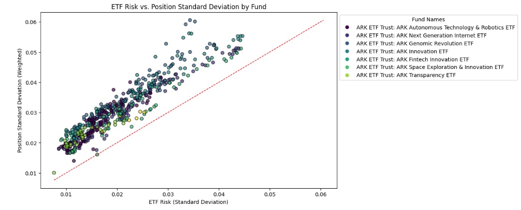
The plot highlights:
- ETF Risk vs. Position Risk: Points are color-coded by fund names to distinguish them visually.
- Diagonal Reference Line: A dashed line marks equal values for ETF and position risks, providing context for evaluating deviations.
Insights
The visualization provides a clear perspective on how risk is distributed across funds, helping identify outliers or trends in ETF management.
# Connect to WRDS
conn = wrds.Connection()
sql_query = '''

with etf_risk as (
select h.report_dt
	, fund_name
	, cusip8
	, stddev(d.ret) as etf_risk
FROM crsp.fund_hdr f
inner JOIN
    crsp.holdings AS h
    ON f.crsp_portno = h.crsp_portno
inner join
	crsp.dsf d on d.cusip = f.cusip8  and d.date between h.report_dt - INTERVAL '252 days' AND h.report_dt
where mgr_name = 'Catherine D. Wood' and mgmt_name = 'ARK Invest'
group by  h.report_dt
	, fund_name
	, cusip8
order by stddev(d.ret) DESC),

risk_port as (
SELECT
	h.report_dt,
    f.fund_name,
    h.security_name,
    h.cusip,
    (h.percent_tna/100) as percent_tna,
    STDDEV(d.RET) as position_std_dev
FROM
    crsp.fund_hdr AS f
inner JOIN
    crsp.holdings AS h
    ON f.crsp_portno = h.crsp_portno
inner join
	crsp.dsf d on d.cusip = h.cusip  and d.date between h.report_dt - INTERVAL '252 days' AND h.report_dt
WHERE
    f.mgr_name = 'Catherine D. Wood' and mgmt_name = 'ARK Invest'
    --and f.fund_name ='ARK ETF Trust: ARK Innovation ETF'
    --and h.report_dt = '2014-12-31'
group by h.report_dt,
    f.fund_name,
    h.security_name,
    h.cusip,
    h.percent_tna
)
select e.report_dt,
	e.fund_name,
	e.etf_risk,
	SUM(p.position_std_dev* percent_tna) as position_std_dev
from etf_risk e
	inner join risk_port p on p.report_dt=e.report_dt and p.fund_name=e.fund_name
group by  e.report_dt,
	e.fund_name,
	e.etf_risk
'''
etf_risk = conn.raw_sql(sql_query)

# Close the WRDS connection
conn.close()
import matplotlib.pyplot as plt
import pandas as pd


# Encode fund names as numerical values for color mapping
fund_names, fund_labels = pd.factorize(etf_risk['fund_name'])

# Plotting
plt.figure(figsize=(10, 6))
scatter = plt.scatter(
    etf_risk['etf_risk'],
    etf_risk['position_std_dev'],
    c=fund_names,  # color by fund_name
    cmap='viridis',  # color map
    alpha=0.7,
    edgecolor='k'
)

# Add a diagonal line
min_val = min(etf_risk['etf_risk'].min(), etf_risk['position_std_dev'].min())
max_val = max(etf_risk['etf_risk'].max(), etf_risk['position_std_dev'].max())
plt.plot([min_val, max_val], [min_val, max_val], 'r--', linewidth=1, label='Equal Line')

# Custom legend
legend_handles = []
for i, fund_name in enumerate(fund_labels):
    legend_handles.append(plt.Line2D([0], [0], marker='o', color='w', markerfacecolor=scatter.cmap(i / len(fund_labels)), markersize=8, label=fund_name))
plt.legend(handles=legend_handles, title='Fund Names', loc='upper left', bbox_to_anchor=(1, 1))

# Labels and title
plt.xlabel('ETF Risk (Standard Deviation)')
plt.ylabel('Position Standard Deviation (Weighted)')
plt.title('ETF Risk vs. Position Standard Deviation by Fund')

plt.show()

Comments by rgcarrol